When working with long lists or wide tables, it is easy to lose track of headers or important labels as you scroll. Google Sheets has a Freeze feature that keeps specific rows or columns visible at all times. This makes it more convenient to read your data and much more efficient to work with.
![]()
In one of our best selling template, we used freezed rows to create a top panel that act as control centre. This enhances user experience, making it easy for users to set their preferred setting before starting to use their social media tracker.
How to Freeze Rows
To freeze 1 or more rows, follow steps below.
- Go to the top menu and click "View".
- Select "Freeze".
- Choose one of the following options:
-
1 row → keeps the first row visible when scrolling.
-
2 rows → keeps the first two rows visible when scrolling.
- Up to row X → (more flexible) freezes all rows above and including the active cell.
-
How to Freeze Columns
To freeze 1 or more columns, follow these steps:
- Go to the top menu and click "View".
- Select "Freeze".
- Choose one of the following options:
-
1 column → keeps the first column visible when scrolling.
-
2 columns → keeps the first two columns visible when scrolling.
-
Up to column X → freezes all columns to the left of and including the active cell.
-
How to Unfreeze Rows or Columns
If you want to remove the freeze:
- Go to View > Freeze.
- Select No rows or No columns.
The sheet will return to normal scrolling without any frozen rows or columns.
If you prefer to dive deeper into this topic, we highly recommend reading Ben Collin's article that covers how to freeze rows or columns using appscript.